1 Introduction
This technical note summarizes the results of a series of tests performed with an implementation of APDB which uses Apache Cassandra as a backend. It is a continuation of the previous tests with relational databases which were described in DMTN-113. Those tests showed serious scalability issues which practically rule out use of that technology in a production setup. Scaling performance to acceptable level will likely need a distributed system that has larger aggregate I/O throughput and IOPS and uses RAM for faster data access.
Apache Cassandra is a popular NoSQL database system with a number of attractive features that can help with the implementation of such scalable system:
- it is an inherently distributed system with a flexible and configurable partitioning of the data,
- partitioning and clustering of on-disk data can be utilized to minimize the number of I/O requests when reading the data,
- all new data is stored in RAM (and a fast commit log) making write operations extremely fast,
- configurable replication and data consistency supports a range of trade-offs between performance and data consistency.
These Cassandra features seem to be a close match for the requirements of the APDB system, and to validate that it can deliver necessary performance we implemented series of tests using a small-scale Cassandra cluster.
2 Hardware
It was clear before we started this round of experiments that we need a reasonably large cluster to obtain meaningful performance numbers. While Cassandra can run on a single node, it is clearly not an optimal setup for the scale of the problem; some features such as replication cannot be even used with a single node cluster. For reliable consistency Cassandra should use a replication factor three, which needs at least three-node cluster, though this is not optimal for performance because each node has a full set of data.
As we did not have dedicated server hardware for APDB testing, we had to borrow three machines from the PDAC QServ cluster:
- one machine from the existing QServ cluster used initially as QServ czar node with full name lsst-qserv-master02 (using short name master02 below),
- two new identical machines purposed for a newer QServ cluster purchased in 2019.
Here is the summary table with the most important specs:
| master02 | master03,04 | |
|---|---|---|
| CPU | 2 x Intel Xeon Gold 5120; 2 x 14 cores | 2 x Intel Xeon Gold 5218; 2 x 16 cores |
| RAM | 256 GiB | 256 GiB |
| Storage | 12 x 480 GB SATA SSD; RAID controller | 5 x 4000 GB NVMe SSD |
One significant difference between old master02 and new master03,04 machines is their storage systems: the old machine has slower SATA storage connected to a single RAID controller. This limits performance of the storage, in particular IOPS. Here are the approximate aggregate numbers for SSD storage as a whole on two types of hardware:
| master02 | master03,04 | |
|---|---|---|
| Read IOPS | 15 k | 1.5 M |
| Write IOPS | 12 k | 1.1 M |
| Read bandwidth | 2.3 GBps | 8.5 GBps |
| Write bandwidth | 4.5 GBps | 8.5 GBps |
There was no dedicated study of the impact of the lower IOPS rate (master02) on the performance of the whole Cassandra cluster.
3 Client configuration
Testing was done using the same ap_proto application that was used in earlier
tests. The dax_apdb package that implements the APDB interface was extended to
support a Cassandra backend using the cassandra-driver Python package. The APDB
interface needed a few incompatible changes due to differences in the data model
between relational databases and Cassandra. All development was done on a
separate branch due to that.
Like in previous tests with Oracle, clients were running at the LSST verification cluster using MPI for client communication. There was one client process per single CCD, for a total of 189 clients running concurrently. Clients communicated with the Cassandra cluster using the Cassandra native protocol, with all three server nodes accessible over a public network (except in the case of the Docker test, as described below).
4 Partitioning
Partitioning and clustering indices play a very important role in Cassandra, and need to be carefully chosen based on how data are produced and accessed. For the AP pipeline, the main access method is based on spatial coordinates; each client needs to read data corresponding to a whole CCD region and produces new data for the same region. Access to DIASource and DIAForcedSource is also restricted by a history depth limit (nominally 12 months). For non-source data, it is obvious that we need some sort of spatial partitioning. For sources, it likely will be a combination of spatial and temporal partitioning.
One of the goals of partitioning in a distributed system like Cassandra is to optimally distribute load across multiple nodes in the cluster, in order to avoid bottlenecks. In the context of the AP pipeline, with 189 independent per-CCD processes, this means that we want to send queries from different CCDs to different partitions. Ideally, we would want a one-to-one correspondence between CCDs and partitions, but that is of course impossible because CCD position and orientation on the sky is random. The goal therefore is to optimize the size of the partition and partitioning scheme, so that on average the load is balanced across the cluster and performance is optimal.
4.1 Spatial partitioning
For spatial partitioning, we could select one of the existing schemes already in use in LSST, e.g. HTM or Q3C. It is interesting to compare some characteristics of the partitioning based on these pixelization schemes. For this, we implemented a simple Monte-Carlo experiment with a selected pixelization scheme/level and randomly placing a square CCD regions on the resulting partitioning grid. For each trial, three numbers were calculated:
- number of pixels touched by a single CCD which should corresponds to the number of queries that need to be executed;
- total area of all pixels touched by single CCD, number of DIAObjects returned from queries is proportional to area, and it is beneficial to have this are to be as close as possible to a CCD size;
- number of CCDs touched by a single pixel, this corresponds to the number of clients querying the same partition.
For this exercise, two pixelization schemes were selected – HTM, and MQ3C –
which are implemented in the sphgeom package. Plots below summarize the results of
the Monte-Carlo. Figure 1 shows average values of
the two numbers as a function of level. Figure 2
shows distribution of the values for specific level.
Figure 3 shows distributions for number of
pixels per CCD (tile) and total area of those pixels.
From the plots one can conclude that MQ3C shows significantly better behavior for the pixels-per-tile value, while for tile-per-pixel value they behave similarly. This is an expected behavior due to differences in pixel shape.

Figure 1 Average number of pixel/tile connections as a function of pixelization level for different pixelization schemes.
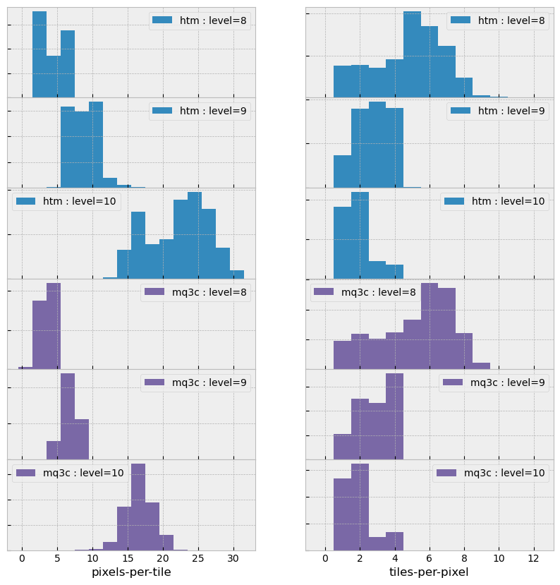
Figure 2 Distributions for the number of pixel/tile connections for different pixelization schemes and pixelization level.
Figure 3 Distributions for the number of pixels per tile and total pixel area for different pixelization schemes and pixelization level.
4.2 Temporal restriction
Queries on the DIASource table are temporally restricted to 12 months. There are a few different strategies that may be used for handling this restriction. One important goal in defining a schema for APDB is to eliminate the need to access files that were produced a long time ago (older than 12 months), so that those files could be moved to slower, less expensive storage.
Possible options for schema definition to satisfy this goal:
- Partition by spatial index only, cluster using temporal index. This does not increase the number of partitions or queries, but it means that old SSTable files have to be searched for data they don’t have.
- Partition by both spatial and temporal index. This means increasing the number of partitions and queries. Due to Cassandra’s probabilistic indexing feature, it may still happen that some old files may be accessed.
- Using client-controlled namespaces, probably easiest in the form of separate tables. Management of the namespaces will be left to client, so some additional logic will need to be implemented. Number of queries will grow depending on the granularity of the namespace “partitioning”.
The latter option is probably the one that allows the most precise control over which data can be retired to slow storage without impacting performance. A few initial tests in this study were done with temporal partitioning, but most of the remaining tests used separate client-controlled tables for namespaces with a one-month granularity of the namespaces.
5 Tests with Cassandra on PDAC
Below is a description of multiple tests performed with a Cassandra cluster running on three PDAC nodes. Tests were done with different setups and configurations; not all results of these tests are meaningfully comparable to other results due to configuration differences or mistakes that were a part of learning process. Cassandra configuration is quite complicated and needs a deep understanding of Cassandra’s internal architecture, so trial and error is an essential part of the process. There are a lot of details about the tests in the corresponding JIRA tickets; links are included below.
5.1 Initial test
The very first test (DM-20580) was done mostly to study the tools, configuration, and the behavior of the system with some specific goals:
- check initial performance numbers
- understand configuration and find optimal parameters for our setup
- evaluate management tools and how they can be integrated into workflow
In this initial test, three nodes were configured slightly differently to take into account differences in their storage systems. In particular, the master02 node was allocated 96 tokens compared to 256 for each of the other nodes, which reduced data volume stored on that node and correspondingly the load on that host.
One of the early ideas was to try to keep the number of I/O operations minimal by not flushing the data from memory during the night, then forcing the flush and compacting data during the day. Implementing this cycle in this initial test did not show any improvements in performance with compacted data compared to a default setup when data was compacted less frequently. Our intermediate conclusion was that Cassandra shows no significant performance degradation with less compacted data, so the default compaction policy may work sufficiently well. Forced compaction takes significant time and there is no reason for doing it without clear benefit.
Overall performance of this initial test was unexpectedly low. After running for 30k visits (~1 month worth of data), average read time was at the level of 3 seconds per one CCD per visit, but average store time was around 7 seconds. This did not make a lot of sense, as Cassandra performance for write operations was supposed to be much better. Also during the test, we observed many cases of client-side timeouts that pointed to significant performance issues that had to be understood.
To analyze these performance issues, we instrumented our Cassandra setup
with a monitoring tool that used the Cassandra JMX interface (DM-23604) in order to
extract monitoring metrics and dump them to a file which was later ingested into
InfluxDB and exposed to Grafana. Monitoring information was also extracted
from the ap_proto log files and saved to the same InfluxDB so we could
correlate things happening on both the client and server sides.
Analyzing the monitoring data, we quickly established that the reason for poor performance in the initial test was over-commitment of memory. Even though the JVM was configured to leave a significant amount of RAM to other processes, there were some services (notably GPFS and Docker) which also needed a significant amount of RAM and this caused intensive swapping. Reducing memory allocation for the JVM allowed us to avoid swapping and improved performance to more reasonable level.
5.2 Java Garbage Collection
The second round of tests (DM-23881) started with a reduced JVM memory allocation (160 GB) which eliminated swapping, but we still saw frequent timeouts on the client side. Monitoring showed that on the server side there were significant delays happening during garbage collection. Apparently, the default garbage collection algorithm (ParNew+CMS) used by Cassandra is not optimal for large memory systems. Switching to to a different algorithm (G1GC) improved GC efficiency and fixed client-side timeouts; this was done after ~60k visits, the effect is clearly seen on the plot below.
Two other significant changes at this step were:
- avoiding spatial filtering on server side (which uses a fine-grain HTM20 index) to drastically reduce the number of queries executed on the server, data from the whole partitions is now returned to the client;
- switching to MQ3C level 10 pixelization for partitioning, this reduces the size of the partitions and the amount of data per CCD that are returned to client (see Figure 3)
With this setup the test was run for 180k visits (approximately 6 months). Write performance improved dramatically, and database operations were now dominated by read time which grows approximately linearly with the visit number. Figure 4 summarizes read performance for all separate tables and their total. At 180k visits, total read time is approximately 10 seconds per visit (per CCD).
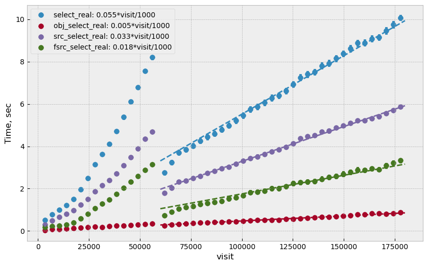
Figure 4 Select execution time as a function of visit number, “obj_select_real” is time for DIAObject table, “src_select_real” is for DIASource, “fsrc_select_real” is for DIAForcedSource, and “select_real” is the sum of three times. Data for visits below 60k is not included in fits.
This test was configured without replication, and with equal numbers of tokens on each node, meaning each node was serving one third of the total data. In a production setup, we will have more than one replica for high availability reasons. Replication configuration needs to be tested as well, even though a three-node cluster is not ideal for scaling the number of replicas. Cassandra has a so-called tunable consistency feature, which allows certain tradeoffs between data consistency and performance; the mechanism depends on the number of replicas in the cluster. A minimal sensible replication level for this mechanism is three if high availability is required.
For the next test, configuration was set to use two replicas, though the consistency
level was kept at ONE. The main goal of this setup was to verify that the
cluster could handle twice the throughput in I/O without degradation, and there
was a concern that replication level three in cluster of three machines is not
optimal. With this setup, ap_proto ran for 100k visits. It showed the same
linear scaling for select time without degradation compared to previous test.
Store time stays approximately constant or even improves slightly over time.
Figure 5 shows select time as a fitted function of
visit number, Figure 6 is a fit of store time for
four tables (DIAObject data is stored in two separate tables). Store time is
significantly lower than select time, just as expected due to Cassandra
storing its data in memory.
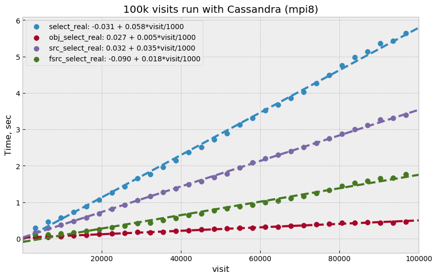
Figure 5 Select execution time as a function of visit number, labeling corresponds to previous plot.
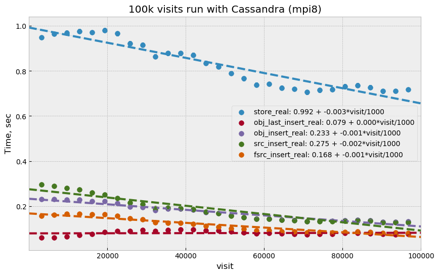
Figure 6 Store execution time as a function of visit number. Total time is higher than the sum of individual tables due to additional overhead on client side for query preparation.
5.3 Test with docker
For the next series of tests (same ticket DM-23881), it was decided to run multiple Cassandra instances on a single physical machine, one instance per storage disk. SSD storage on master02 was organized into 4 virtual disks, and they were all connected to single RAID controller which could limit overall performance. The total number of Cassandra nodes in this cluster configuration thus equaled 14 (4+5+5), and each node was run in a Docker container. One complication with this setup was that we could only map a single docker container to a public routable interface on a host machine (Cassandra default build does not support different port numbers) which means that only three out of 14 nodes could serve as coordinator nodes introducing potentially uneven load into the system.
The goal of this exercise was two-fold:
- Reduce memory allocation per node which should potentially reduce garbage collection overhead in JVM;
- run with replication factor three to check higher consistency level settings.
On the client side, consistency level was set to QUORUM, meaning
at least two replicas had to respond for each operation before success
status was returned to the client.
Like in the previous test, ap_proto was left running for 100k visits with
this configuration. Results are represented in two plots below. Write
performance was improved somewhat in this case, but select performance was about
50% slower compared to the previous result.

Figure 7 Select execution time as a function of visit number for test with Docker.
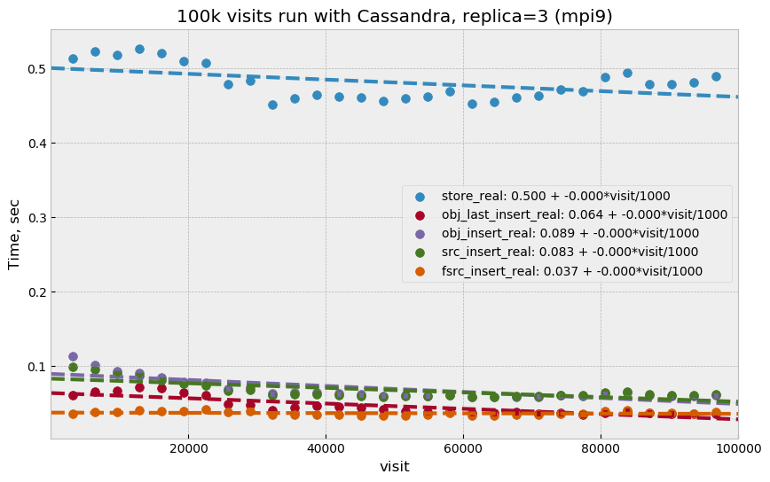
Figure 8 Store execution time as a function of visit number for test with Docker.
5.4 Scylla test
There exists an alternative open source implementation of the Cassandra database -
Scylla. Scylla is implemented in C++, though for compatibility some pieces
(e.g. JMX) run inside a separate JVM instance. The client side “native” protocol is
100% compatible with Cassandra, so existing client code in ap_proto
can run seamlessly with Scylla.
For the next series of tests (DM-24692), we replaced the Cassandra cluster with a similarly configured Scylla cluster with three nodes. Configuration is mostly compatible, though some options behave differently or are not supported. Some special tuning was necessary to avoid memory swapping issues. Scylla was running stably for most part, though on the client side there were occasional transient connection issues observed which did not cause fatal errors.
For the initial test with Scylla we used single replica, with the goal to establish a baseline similar to the Cassandra case. A difference with the Cassandra case was in storage configuration; Scylla does not support multiple data directories, so all data in this test were store on a single physical disk (or one virtual disk in case of master02). A total of 150k visits were produced in this configuration. Plot Figure 9 shows select time dependency, which is consistent, or maybe slightly worse, than the single replica Cassandra case (Figure 4). Store time (Figure 10), like in the Cassandra case, is also negligible compared to select time.
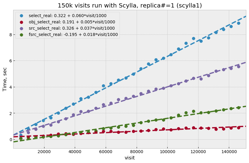
Figure 9 Select execution time as a function of visit number for Scylla with single replica.
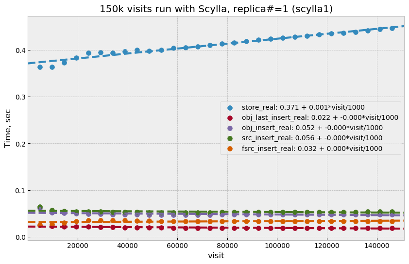
Figure 10 Store execution time as a function of visit number for Scylla with single replica.
For the second round of Scylla tests, it was configured with three replicas and three nodes, so that each node had full set of data. All storage on each node was merged into a single logical LVM RAID0 volume.
Plot Figure 11 shows select performance for this test. Compared to other cases, the behavior looks more complicated – initially select time grows faster, then it suddenly improves around visit 90k. That improvement corresponds to a restart of the Scylla cluster that was performed as a cleanup after a GPFS outage. Scylla does not use GPFS, so it is not clear how any potential GPFS issues could have affected Scylla. A more likely explanation is that Scylla itself developed some inefficiencies that were cleared after restart.
Compared to the three-replica Cassandra case, Scylla performance (after restart) is somewhat better, ~7 vs ~9 seconds at 100k visits.
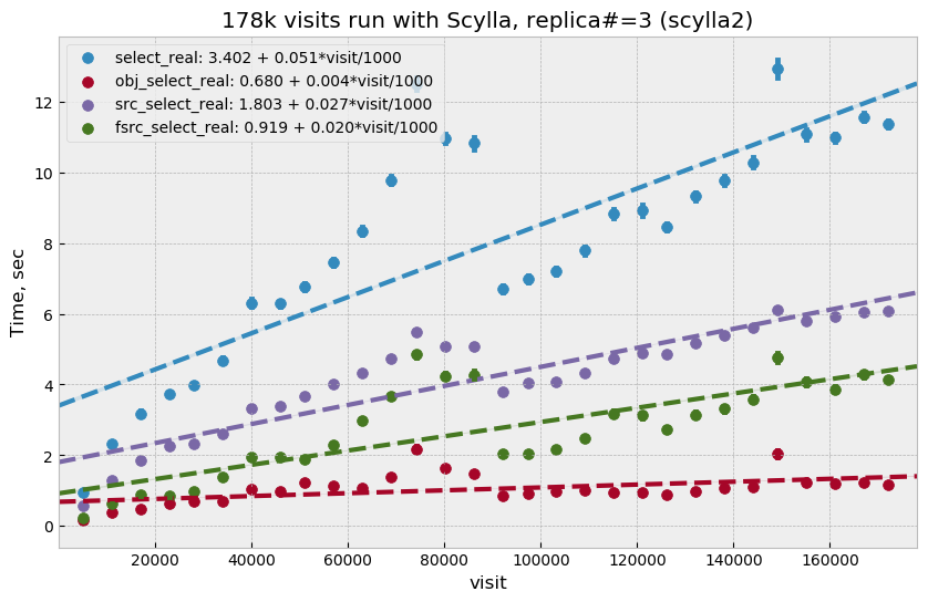
Figure 11 Select execution time as a function of visit number for Scylla with three replicas.
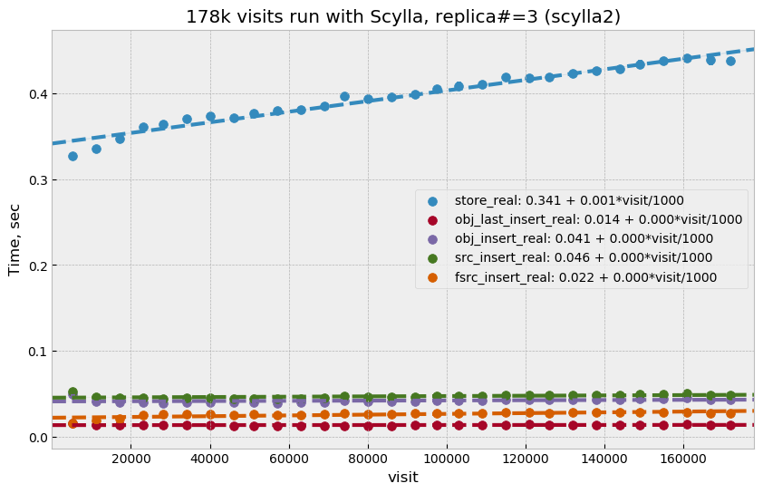
Figure 12 Store execution time as a function of visit number for Scylla with three replicas.
5.5 Three-replica Cassandra test
For the final test, we repeated the Cassandra test with three replicas but without
Docker, using three instances similar to Scylla case, and with an identical
storage setup (DM-25055). One of the goals of this test was to check how
consistency level affects performance, so part of the test was run at
consistency level ONE for reading (and QUORUM for writing).
Plot Figure 13 shows select timing
for the first 180k visits when consistency level for reading was set to
QUORUM. Performance is significantly slower than for Scylla, and also
slower than Cassandra performance with three replicas in the Docker setup. Plot
Figure 14 shows timing for the last 10k
visits when reading consistency was set to ONE. For this case performance
was closer to what was seen with Scylla and the earlier Docker test, but in both
those cases consistency was set to QUORUM.
It is not clear why Cassandra performance differs so much between a Docker setup with 14 nodes (which is sub-optimal) and a 3-node configuration. We tried to monitor query tracing information provided by Cassandra, and there seemed to be an indication that query execution on master02 was taking longer than on the two other hosts, though exact numbers are hard to interpret due to the large number of concurrent clients. There was also some indication that the replica repair mechanism may be responsible for some of this effect; this can be investigated further.
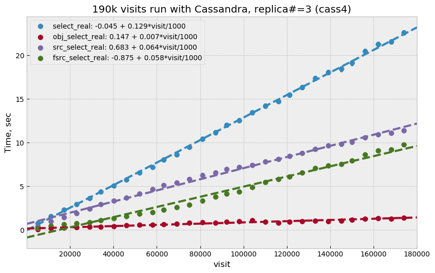
Figure 13 Select execution time as a function of visit number for Cassandra with three
replicas and read consistency level QUORUM.

Figure 14 Store execution time as a function of visit number for Scylla with three
replicas and read consistency level ONE.
5.6 Summary
It is hard to summarize all of the above results in one single metric. For our use case, the bottleneck seem to be the execution time of the select queries, so we chose this as a main parameter. In most cases this parameter grows linearly with visit number, except for the case of Scylla with three replicas which has some unexplained fluctuations. It is expected to grow with the size of the data, and due to the maximum source history size of 12 months it should level off after that time.
For summary, we want to present the numbers that can be compared easily, so we chose as a metric the time to read all tables at after 180k visits (about 6 months of data). Not all of the above tests generated a full 180k visits; for those that did not we include an estimate obtained from extrapolating fitted data.
Here is the summary table for all of the above tests:
| Test type | #replicas | Time, sec |
|---|---|---|
| Cassandra | 1 | 10 |
| Cassandra | 2 | 10.5 |
| Cassandra w/Docker | 3 | 17 |
| Scylla | 1 | 11 |
| Scylla | 3 | 12.5 |
| Cassandra w/QUORUM | 3 | 23 |
| Cassandra w/ONE | 3 | 15 |
6 Data sizes
For reference here, is the size of the data on disk for some of the test cases (total size for all instances):
| Test type | #replicas | #visits | Size, TB |
|---|---|---|---|
| Cassandra w/Docker | 3 | 100k | 5.8 |
| Scylla | 1 | 150k | 3.03 |
| Scylla | 3 | 178k | 10.7 |
| Cassandra | 3 | 190k | 11.1 |
The numbers are consistent and approximately correspond to 2 TB per replica per 100k visits.
7 Unresolved questions
A lot of information was collected during all these tests, but still there are some question that have not been answered completely. Here are some questions/ideas worth investigating in the future tests:
- It is not entirely clear why select time is proportional to the data volume (or visit number). Naively, it would seem that the data volume is not extremely large and time should probably be proportional to the number of I/O operations which itself ideally should remain approximately constant.
- Efficiency of the client side operation was not measured. It may be significant (10-20% or larger) and may have various contributions; there may be an opportunity for optimization there too.
- Scylla numbers look good and maybe too good. It may be possible that Scylla uses some shortcuts which optimize performance but may hurt consistency. This needs to be understood if we think that Scylla is a viable option.
- It is not clear how the master02 storage system affected overall performance. There are indications that a bottleneck may be there. For future tests it would be better to have a more uniform setup.
- There are indications that concurrent reads/writes cause “read repairs” in Cassandra, which is a potentially costly operation. It would be nice to be able to quantify this and try to reduce it.
8 Conclusion
The tests show that a small-scale Cassandra cluster can provide better performance for storing APDB data than a single-node (or Oracle RAC) relational database server. The main attractive feature of Cassandra is the ability to scale performance horizontally by simply extending the existing cluster. This scalability needs to be tested in more realistic setup than our present test cluster.
Based on this experience, future tests with Cassandra can benefit from using hardware which better matches the Cassandra workload:
- The JVM seems to work better with smaller resident sets; in that respect it may be better to have larger number of hosts with smaller RAM than a single host with huge memory.
- High IOPS seem to be critical for achieving good read performance with APDB data, so it is advisable to have all live data on NVMe disks which provide much better concurrency than SATA disks.
There are a lot of unanswered questions outlined in the previous section; answering them in the future tests can improve our understanding of bottlenecks and further improve performance.